Birdsong Classification Project
Complete Python and ML pipeline for bird song classification, enriched with presentation insights, conclusions, and visuals from the original slides.
- published
- reading time
- 4 minutes
🐦 Birdsong Classification Project — Complete Version
In this blog post, we’ll explore how to automatically classify bird species from their songs using audio analysis, signal processing, and machine learning.
This project merges the original technical pipeline with insights, visuals, and conclusions from the “Birdsong Classification Project” presentation.
🎶 Why Birdsong Classification?
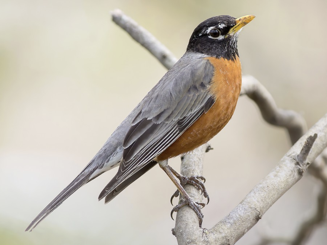
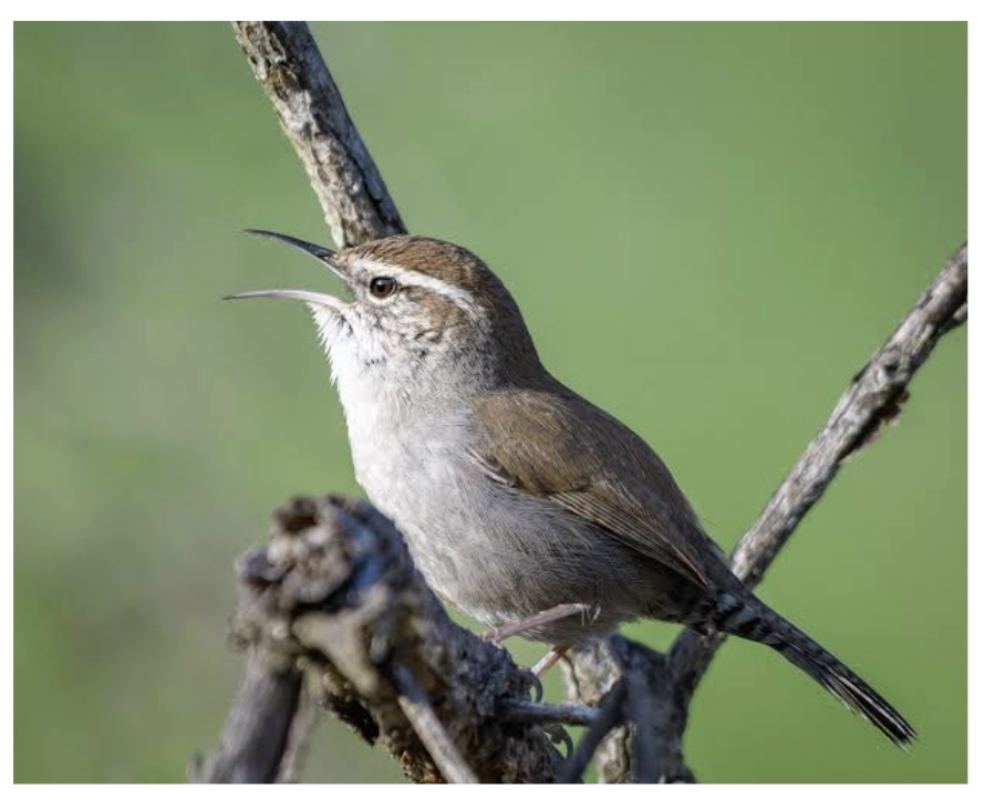
Bird songs are unique to each species.
With Machine Learning, we can analyze their sound signatures to automatically recognize the corresponding species.
Objectives:
- Identify species from their songs.
- Obtain an accurate and robust model.
- Contribute to automated biodiversity monitoring.
Key points:
- 5 species studied
- Focus: American continent
- About 5000 audio samples

🌍 Overview
Birdsong classification plays a crucial role in:
- Ecological monitoring — tracking biodiversity and population trends.
- Citizen science — leveraging crowd-sourced recordings like Xeno-Canto.
- Automated surveys — detecting species in remote regions.
We rely on two key datasets:
🎯 Project Objectives
- Extract audio features (MFCC, ZCR, Spectral Centroid).
- Preprocess audio (filtering, normalization, silence trimming).
- Train and evaluate ML models (Random Forest, LightGBM, PyCaret).
- Visualize spatial and spectral data for interpretation.
🛠️ Tools & Libraries
- Python 🐍
- Librosa, NumPy, Pandas for feature extraction
- Scikit-learn, LightGBM for ML
- Seaborn, Matplotlib, Folium for visualization
🎵 1. Loading and Preparing Data
We begin by installing dependencies and loading metadata.
import os, librosa, numpy as np, pandas as pd
import seaborn as sns, matplotlib.pyplot as plt
from sklearn.model_selection import train_test_split
from sklearn.ensemble import RandomForestClassifier
from sklearn.metrics import classification_report, confusion_matrix
import scipy.signal
from pycaret.classification import *
df = pd.read_csv("./bird_songs_metadata.csv")
df['path'] = df['filename'].apply(lambda x: os.path.join("wavfiles", x))
df.sample(5)
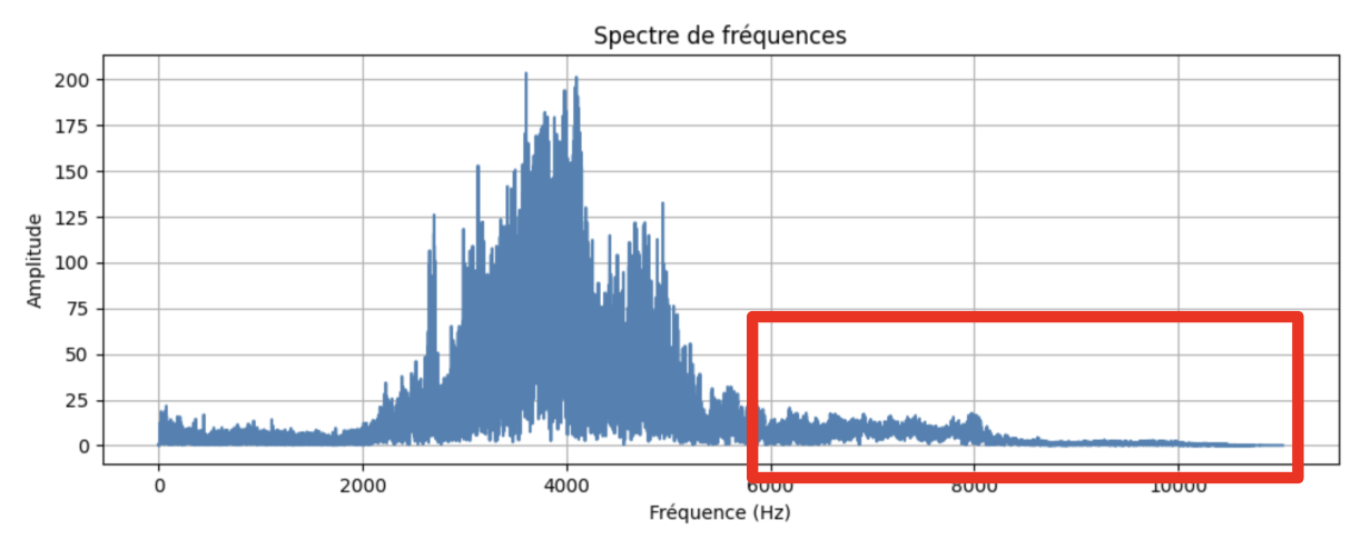
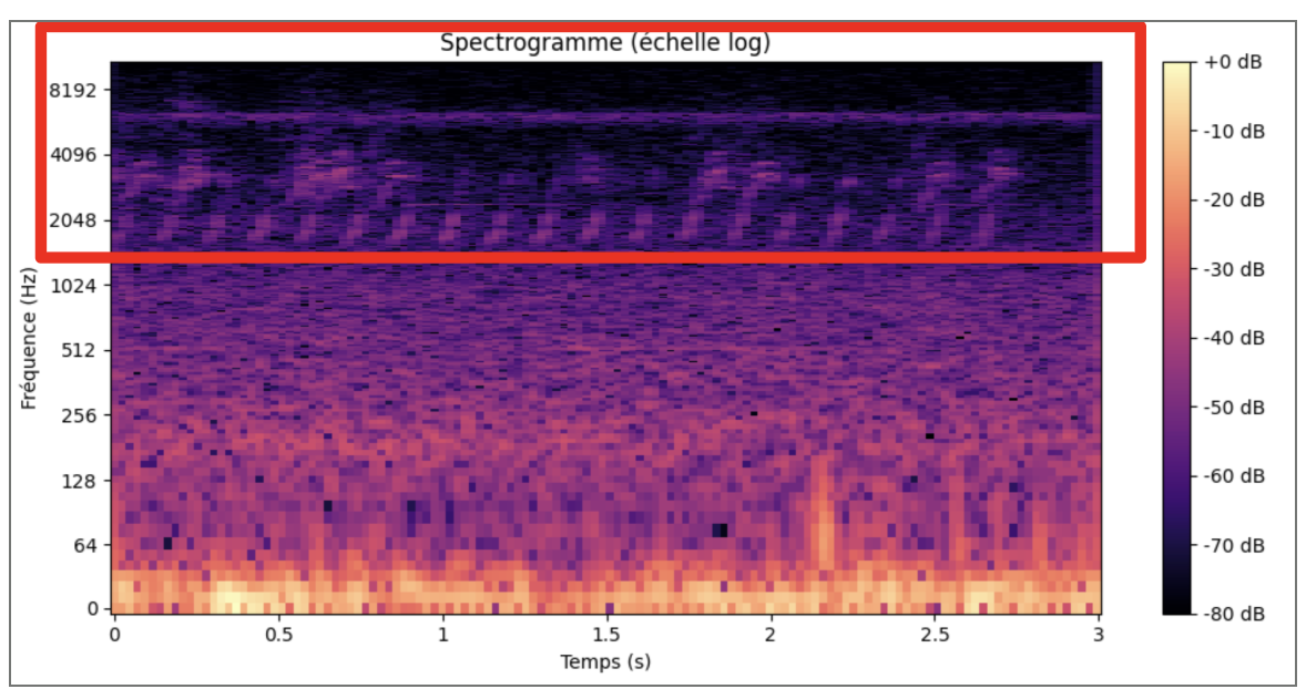
🎚️ 2. First Audio Analysis
First sound analysis:
- Blue: frequencies and amplitudes
- Purple: frequency evolution over time
Conclusion:
- Poor quality samples
- Lots of background noise
- Large amplitude disparity
🔧 3. Audio Preprocessing
To make the data usable, we perform:
- Frequency filtering
- Volume normalization
- Silence trimming
def extract_clean_features(file_path):
  y, sr = librosa.load(file_path, sr=22050, duration=5.0)
  low, high = 200/(sr/2), 10000/(sr/2)
  b, a = scipy.signal.butter(2, [low, high], btype='band')
  y = scipy.signal.filtfilt(b, a, y)
  y = librosa.util.normalize(y)
  y, _ = librosa.effects.trim(y, top_db=15)
  mfcc = librosa.feature.mfcc(y=y, sr=sr, n_mfcc=13)
  zcr = librosa.feature.zero_crossing_rate(y=y)
  centroid = librosa.feature.spectral_centroid(y=y, sr=sr)
  return np.hstack([np.mean(mfcc, axis=1), np.std(mfcc, axis=1), np.mean(zcr), np.mean(centroid)])
Goal: keep the essential sound and remove background noise.
🌲 4. Model Training — Random Forest
X_train, X_test, y_train, y_test = train_test_split(X, y, stratify=y, random_state=42)
clf = RandomForestClassifier(n_estimators=100, random_state=42)
clf.fit(X_train, y_train)
y_pred = clf.predict(X_test)
print(classification_report(y_test, y_pred))
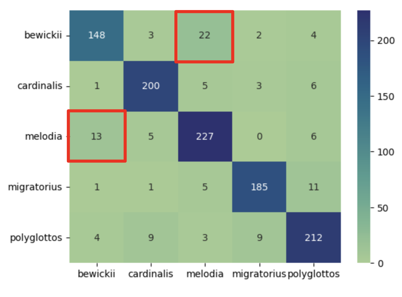
Results:
- Good overall result
- Average accuracy: 0.90
- Some confusion between similar species
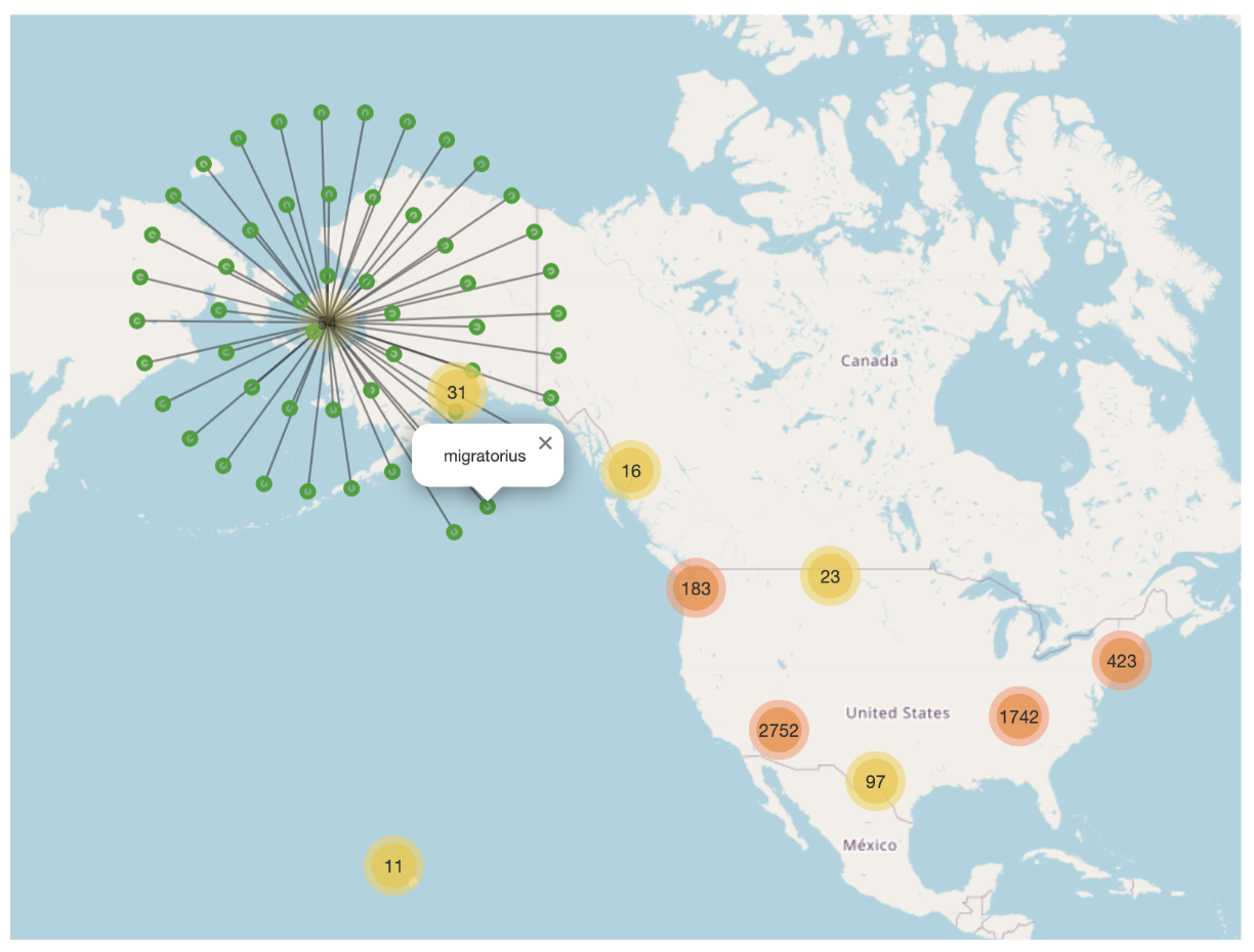
🗺️ 5. Geographic Analysis
To better understand our dataset, we clean and visualize location data.
df_clean = df.dropna(subset=['latitude', 'longitude', 'altitude'])
Conclusion:
- Presence of geographic clusters of species
- Latitude/longitude influence the models
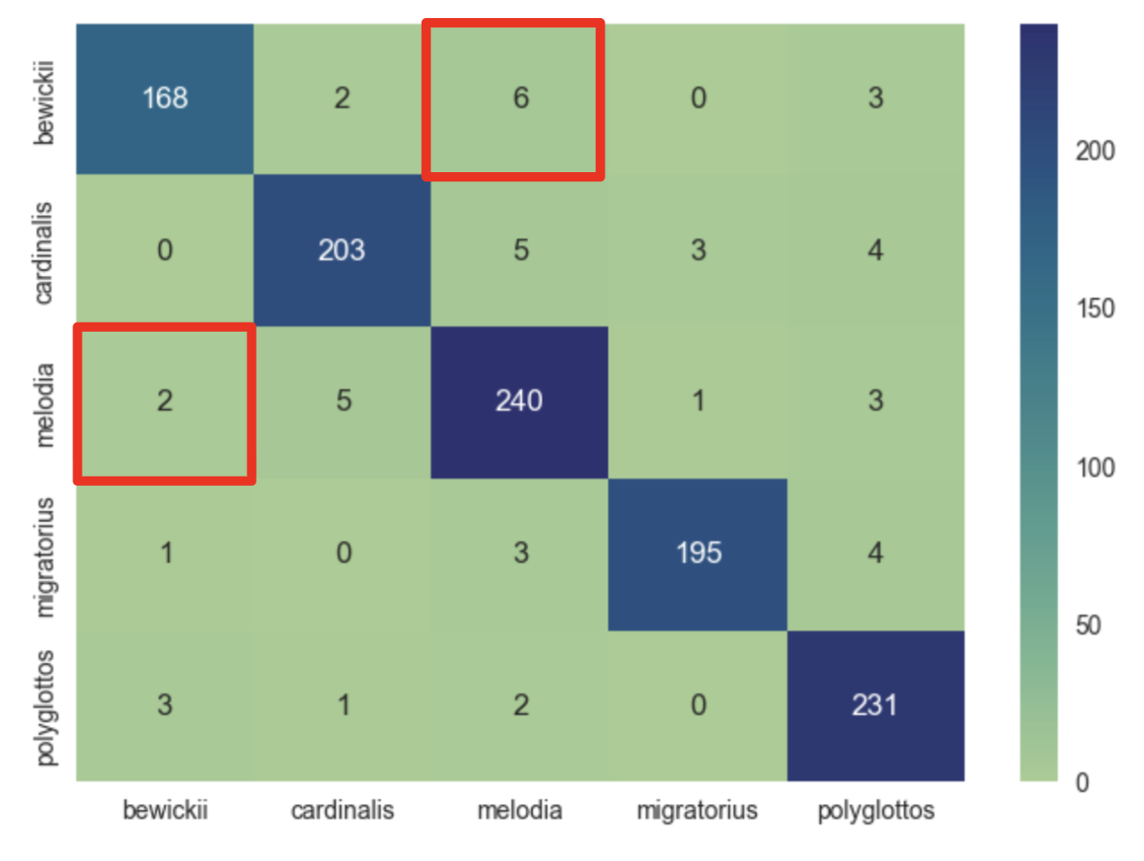
⚡ 6. Improved Training with Geospatial Features
We add geographic coordinates to our cleaned audio features.
Features:
- Cleaned audio samples
- Altitude
- Longitude
- Latitude
Improvements:
- Accuracy: 0.90 → 0.96
- Fewer inter-species confusions
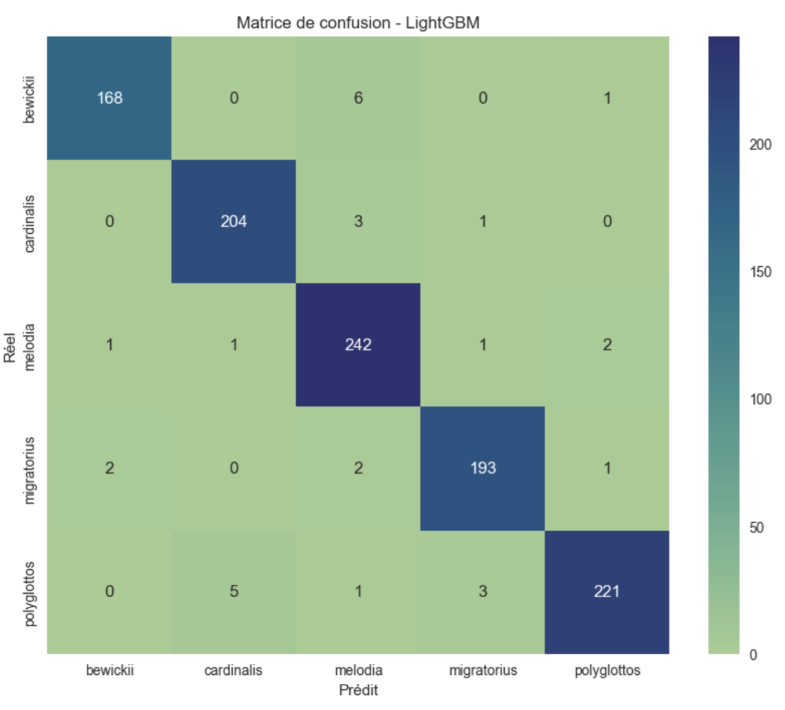
🚀 7. Model Upgrade — Light Gradient Boosting Machine
After comparing models via PyCaret, we switch to LightGBM for optimization.
Split:
- 60% Training
- 20% Test
- 20% Validation
import lightgbm as lgb
model = lgb.LGBMClassifier(n_estimators=500, learning_rate=0.05, num_leaves=40, max_depth=10, random_state=42)
model.fit(X_train, y_train)
Result:
- Accuracy 0.96 → 0.97
- Slight improvement on rare species
🧩 8. Model Comparison
- Little difference between LGBM and Random Forest.
- Random Forest is ~20× faster.
- Audio cleaning is crucial.
- Geographic features significantly increase accuracy.
Final conclusion:
For a balance between performance, efficiency, and speed,
Random Forest Classifier remains the best option.
![]()
🧠 9. Support & Tools
- Mapping: Folium, MarkerCluster
- Plotting: Matplotlib + Seaborn
- Model 1: Random Forest Classifier
- Model 2: LightGBM
- Audio Analysis: Librosa
- Datasets: Kaggle + Xeno-Canto
🔗 Sources:
🧭 10. Conclusion
🌿 Key Insights
- The audio cleaning and preprocessing stage proved to be the most crucial step in achieving reliable classification.
- Incorporating geospatial features (latitude, longitude, altitude) significantly improved model precision and reduced inter-species confusion.
- The Random Forest Classifier remains the most balanced choice, offering a strong accuracy-to-efficiency ratio.
- While LightGBM achieved slightly higher accuracy, it demands substantially more computational resources — an important consideration for ecological and large-scale deployments.
📊 Model Performance Summary
| 🧠 Model | 🧾 Features Used | 🎯 Accuracy |
|---|---|---|
| Random Forest | Raw audio features only | 0.90 |
| Random Forest + Geo | Cleaned audio + geographic data | 0.96 |
| LightGBM + Geo | Cleaned audio + geographic data | 0.97 |
Final Thought:
This project demonstrates how combining bioacoustic signal analysis with geospatial context allows machine learning models to more accurately identify bird species while maintaining computational efficiency.
In practice, the Random Forest model offers the best trade-off between precision, speed, and sustainability — making it a practical choice for real-world biodiversity monitoring.